Table of Contents

• Introduction
• Understanding the Data Dimensions and Memory Usage
• Techniques for Memory-Efficient Array Processing
  • 1. Load Full In Memory
  • 2. Chunking Data Processing
  • 3. Memory Mapping Large Files
  • 4. Incremental / Online Algorithms
  • 5. Parallel and Distributed Computing
• Benchmarking Different Approaches
• Conclusion
• References

Introduction

When dealing with large array-based datasets —especially multidimensional time-series data— memory usage and performance become key concerns. A typical task might involve calculating the square of all values or computing aggregated metrics across millions of samples, which can easily exceed available memory if not handled properly.

This guide presents practical strategies to process such datasets efficiently using Python, without the need to load everything into memory at once.

Understanding the Data Dimensions and Memory Usage

Assume the dataset is a large 2D array:

• Sampling frequency: 2000 Hz
• Duration: 60 seconds
• Number of spatial points: 6000
• Resulting shape: (6000, 120,000)

Memory Estimation

Assuming data is stored as 64-bit floats (8 bytes per sample):

channels = 6000
sampling_rate = 2000  # Hz
duration = 60  # seconds
samples = sampling_rate * duration  # 120,000 samples

memory_bytes = channels * samples * 8  # bytes for float32
memory_mb = memory_bytes / (1024**2)

print(f"Estimated memory usage: {memory_mb:.2f} MB")

Estimated Memory Usage: ~5.49 GB

This means loading the full dataset into RAM may not be feasible on many machines.

Techniques for Memory-Efficient Array Processing

1. Full Load in memory

def compute_squared_sum_full_load():
    data = np.load(file_path)  # Carga todo el array en RAM
    return np.sum(data ** 2, dtype='float64')

2. Chunking Data Processing

Read and process data in small time-based or column-based chunks to manage memory usage efficiently.

import numpy as np

chunk_size = 2000  # 1 second worth of samples
total_chunks = samples // chunk_size

def compute_squared_sum_chunked(file_path):
    squared_sum = 0.0
    for chunk_idx in range(total_chunks):
        data_chunk = read_chunk(file_path, chunk_idx, chunk_size)  
        squared_sum += np.sum(data_chunk ** 2)
    return squared_sum

3. Memory Mapping Large Files

Use numpy.memmap to map the data to memory without loading everything at once.

import numpy as np

data_memmap = np.memmap('data_array.dat', dtype='float32', 
                        mode='r', shape=(channels, samples))
squared_sum = np.sum(data_memmap ** 2)

This approach is efficient for large files that don’t fit in RAM.

4. Incremental / Online Algorithms

Streaming or online processing avoids loading the whole dataset at once:

def incremental_squared_sum(stream_generator):
    total = 0.0
    for data_chunk in stream_generator:
        total += np.sum(data_chunk ** 2)
    return total

5. Parallel and Distributed Computing

Speed up processing by dividing chunks across CPU cores or machines.

from multiprocessing import Pool

def process_chunk(chunk_data):
    return np.sum(chunk_data ** 2)

with Pool() as pool:
    results = pool.map(process_chunk, chunks_list)
squared_sum = sum(results)

This leverages modern multi-core CPUs effectively.

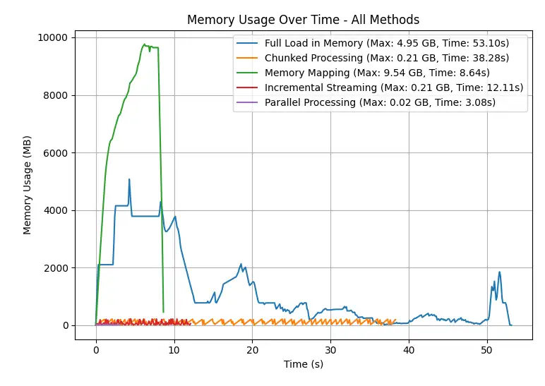
Benchmarking Different Approaches

Method	Peak Memory Usage (GB)	Estimated Time (s)
Full Load in Memory	~4.95	~53.10
Chunked Processing	~0.21	~38.28
Memory Mapping	~9.54	~8.64
Incremental Streaming	~0.21	~12.11
Parallel Processing	~0.02	~3.08

Benchmark example: Calculating square sum on a (6000x120,000) dataset

Note: Please repeat this benchmark on your own machine.
Results may vary depending on system specifications, CPU load, memory usage, and other running processes.

Conclusion

Large 2D datasets, such as time-series matrices with thousands of channels and high sampling rates, can challenge memory limits. Python provides several scalable strategies to process such data without memory overload: chunking, memory mapping, streaming, and parallelization.

These methods make it feasible to compute large-scale operations like squaring values or summing powers efficiently and reliably on commodity hardware.

References

1. NumPy Documentation
2. Python Multiprocessing
3. Repository: Python file